Appreciating R: The Ease of Testing Linear Model Assumptions

Joshua Loong

2019-09-20

data-science

I’d always heard about the package support for traditional statistics in R, but never really had the need or opportunity to dive into it until this year (from working at the amazing Best Buy Canada and the quantitative biology classes I’m taking right now). And while I’m still getting used to it, I’ve been slowly getting a much bigger appreciation for how useful it really can be.

I can say it’s great to use, but I doubt that will sway you if you’re a heavy Python user (as it did not with me) without a really, really concrete example. I hope this example gives you a peek at the potential uses that I myself am still discovering

Assumptions Testing

A HUGE (and I mean HUGE) deal in science is good statistical practice. Without good statistical practice much of the research and insights we produce are useless, and an incredibly important aspect of it is assumptions testing^[1].

All statistical models and tests have underlying mathematical assumptions on the types of conditions upon we can generate reliable results (Hoekstra et al., 2012). What this means is that before we go off and generate predictions, p-values and correlation coefficients, we need to understand whether our data fits certain assumption criteria in order to avoid Type I or II errors given the technique at hand.

This week I’ve been working on an applied biostats assignment, not about linear models directly but made heavy use of them^[2], and came across this wonderful package called gvlma. CRAN link here.

The beauty of gvlma is that it’s a comprehensive, automatic testing suite for many of the assumptions of general linear models. It does both statistical tests and diagnostic plots using an extremely simple implementation for powerful results.

library("gvlma")

model <- lm(y ~ x, data)
summary(gvlma(model))
plot(gvlma(model))

With example outputs of:

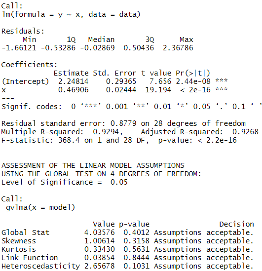
The package is an implementation of a paper by Pena & Slate called Global Validation of Linear Model Assumptions and allows you to quickly check for:

Linearity - the Global Stat tests for the null hypothesis that our model is a linear combination of its predictors^[3].
Heteroscedasticity - the respective stat tests for the null that the variance of your residuals is relatively constant.
Normality - skewness and kurtosis tests help you understand if the residuals of your data fit a normal distribution^[4]. If the null is rejected you probably need to transform your data in some way (like a log transform). This can also be assessed by looking at the normal probability plot it generates.

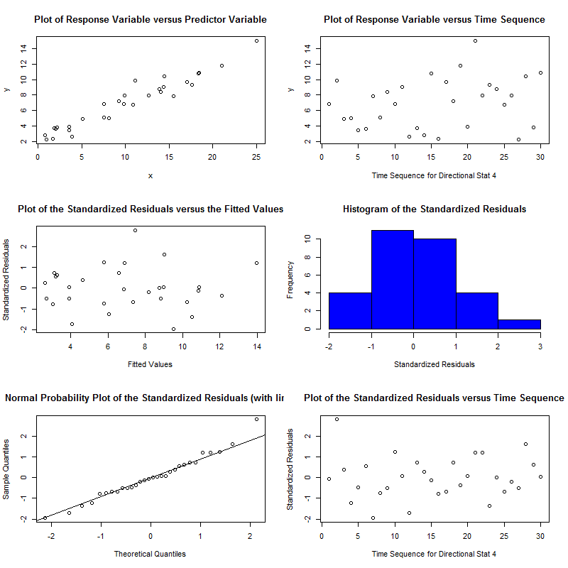
Furthermore, the diagnostic plots also let you understand the relation between your data and these assumptions visually. Other useful capabilities are the link function test which is used for understanding whether the underlying data is categorical or continuous.

As far as I know, there’s no comparable tool suite for models in Python^[5]. There is some support for diagnostics in statsmodels but it doesn’t seem as intuitive to me than what we find here.

But as you can see, this is an incredibly useful package to have for doing traditional statistics. I was blown away with how seamless it was to do this in R. Hopefully this is an interesting example to help push any Python users to try it out 😊

Thanks for reading!

Notes:

[1] The result of poor statistical practice is a huge contributer to the replication crisis we have in multiple fields in the physical and social sciences. You can read more in Shavit & Ellison’s book Stepping in the Same River Twice: Replication in Biological Research.

[2] For those interested, the assignment was in a niche area of applied statistical ecology called critical thermal polygons. Some examples of which can be found in papers by Elliot or Eme & Bennett (2010; 2009).

[3] Made a bit of a mistake here in the first version of the post and /u/OrdoMaas left a nice write up on the intuition behind the corrected linearity assumption:

It’s a common misconception that linearity means that we want to fit a straight line. Instead, it means that we want the model to be a linear combination of the predictors (where linear is used in the linear algebra sense), which is the same thing as saying we want all of our predictors to be added together. This assumption would be violated if the model were, for example, $y = \beta_0 + \exp(\beta_1)X + e$. The relationship between $\beta_0$ and $\beta_1$ would not be additive. On the other hand, a curvy line could be fit by a linear model e.g $y = \beta_0 + \beta_1 \sin(x) + e$. This model satisfies the linearity assumption because there is an additive relationship between $\beta_0$ and $\beta_1$.

[4] Someone pointed out to me that skewness and kurtosis tests may be sensitive to sample size given their experience with the same issue with Jarque-Barea tests, which tests these properties as well. I dug a bit back into the original Slate & Peña paper and they actually did some empirical estimates finding the same thing:

Note that for small sample sizes (n ≤ 30), the asymptotic approximation is not satisfactory… the procedures tend to be conservative.

It may be more useful to use the normal probability plots in small sample scenarios.

[5] These diagnostics are well supported in SPSS, but the world needs to move away from point and click statistics software so I wouldn’t recommend using that. From what I remember, it is also decently supported in SAS for those that use it.

References

Hoekstra, R., Kiers, H., & Johnson, A. (2012). Are assumptions of well-known statistical techniques checked, and why (not)?. Frontiers in psychology, 3, 137.

Peña, E. A., & Slate, E. H. (2006). Global validation of linear model assumptions. Journal of the American Statistical Association, 101(473), 341-354.