Fitting Polynomial Regressions in Python
The linear regression is one of the first things you do in machine learning. It’s simple, elegant, and can be extremely useful for a variety of problems.
But sometimes the data you are representing isn’t exactly linear (in the sense that a straight line would not be the most explanatory of your data), so you’ll need to use something else.
There are a number of non-linear regression methods, but one of the simplest of these is the polynomial regression.
While a linear model would take the form:
A polynomial regression instead could look like:
These types of equations can be extremely useful. With common applications in problems such as the growth rate of tissues, the distribution of carbon isotopes in lake sediments, and the progression of disease epidemics.
Working in Python
Historically, much of the stats world has lived in the world of R while the machine learning world has lived in Python. Given this, there are a lot of problems that are simple to accomplish in R than in Python, and vice versa.
During the research work that I’m a part of, I found the topic of polynomial regressions to be a bit more difficult to work with on Python. Most of the resources and examples I saw online were with R (or other languages like SAS, Minitab, SPSS).
I’m a big Python guy. I love the ML/AI tooling, as well as the ability to seamlessly integrate my data science work into actual software. So even though a lot of the traditional statistics stuff isn’t as straightforward, I wanted to find a working solution in my main language. Hopefully this post will help others in my sitauation.
The beauty of Numpy
If you do some type of scientific computing/data science/analytics in Python, I’m sure you’re familiar with Numpy. For those who don’t know, Numpy is a fantastic Python library whose main focus is on manipulating arrays and matrices.
But it also comes with a series of mathematical functions to play around with data as well. One of which is extremely useful for the topic at hand: the polyfit function.
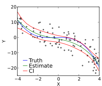
What polyfit does is, given an independant and dependant variable (x & y) and a degree of polynomial, it applies a least-squares estimation to fit a curve to the data.
Here’s a demonstration of creating a cubic model (a degree 3 polynomial):
1 | import numpy as np |
With this above example, you can then give model an array of x-values to get predicted results.
This is simply a redemonstration of what you can find in the Numpy documentation. But what they don’t help you with, either in the documentation or what I could find online, was a guide for model evaluation and significance testing for these regressions.
Model evaluation
To do model evaluation, there was no built in way to do this like there is with other languages (as far as I know). So after some digging I found an awesome way to approach this problem.
Statsmodels is a Python library primarily for evaluating statistical models. It has a number of features, but my favourites are their summary() function and significance testing methods.
Most of the examples using statsmodels are using their built-in models, so I was bit at a loss on how to exploit their great test tooling for the polynomial models we generated with Numpy.
That is until I found this great, and not very well known, function: from_formula.
What you can essentially do is specify the model formula beforehand instead of using the traditional linear OLS regression equation.
According to the documentation this formula can take the form of string descriptions. Most of the examples online looked like this:
1 | import statsmodels.formula.api as smf |
Where you specify the model by using the column names of your pandas dataframe.
But what you can also do, and that was relevant to the work I was doing, is pass to statsmodels a generic equation object which is exactly what we generated in the Numpy example earlier.
Here’s a demonstration bringing it all together:
1 | import statsmodels.formula.api as smf |
This results variable is now a statsmodels object, fitted against the model function you declared the line before, and gives you full access to all the great capabilities that the library can provide.
This includes things like results.summary() which can give a fill regression summary like below:
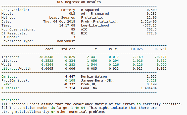
It also gives you things like p-values, R-squared, coefficients, standard error, and tons of other info to help you test whether or not your model is performing well or not. This was a huge revelation for me and I just wanted to share.
Conclusion
I hope this was a good intro on, not just how to build polynomial curves, but also how to pass them to statsmodels for evaluation. This is much easier than having to write your own helper functions to explain your numpy polyfit behaviour.
If you have any thoughts, suggestions, or corrections you can reach out to me @jtloong on Twitter or at joshua.t.loong@gmail.com
Sources
- https://docs.scipy.org/doc/numpy/reference/generated/numpy.polyfit.html
- http://statisticsbyjim.com/regression/curve-fitting-linear-nonlinear-regression/
- https://www.analyticsvidhya.com/blog/2018/03/introduction-regression-splines-python-codes/
- http://www.statsmodels.org/stable/generated/statsmodels.regression.linear_model.OLS.from_formula.html
- http://www.statsmodels.org/devel/example_formulas.html
- https://en.wikipedia.org/wiki/Polynomial_regression
Comments powered by Talkyard.